Shielding calculations were performed with both the deterministic Attila solver and MCNP® using Attila4MC (referred to herein as Attila4MC) simulating an isotropic 60Co gamma point source located at one end of a U-shaped labyrinth lined by iron walls on the outside. Point detector results were generated at the opposite end of the labyrinth using Attila and Attila4MC. Results from a legacy CSG (constructed surface geometry) MCNP calculation were also included in the point detector comparison to validate the unstructured mesh results, generously provided by Richard Haley of TÜV SÜD (https://www.tuvsud.com/en-gb).
Figure 1 shows an XY-cross section of model geometry at the source and detectors’ z-plane. The extent boundaries of the model are 100 x 100 x 100 cm. The isotropic gamma point source is located at coordinates x = -25 cm, y = 30 cm, and z = -50 cm. The U-shaped labyrinth has a 10 cm think iron wall (grey) around the outer boundary. The interior of the labyrinth (green) is modeled as void. Vacuum (non-reentrant) boundary conditions are applied on all other external surfaces. Three point detectors are located on the opposite side of the labyrinth (1, 2, and 3), behind a 10 cm thick aluminum shield (teal). The aluminum shield was divided into four 2.5 cm segments for anisotropic meshing purposes.
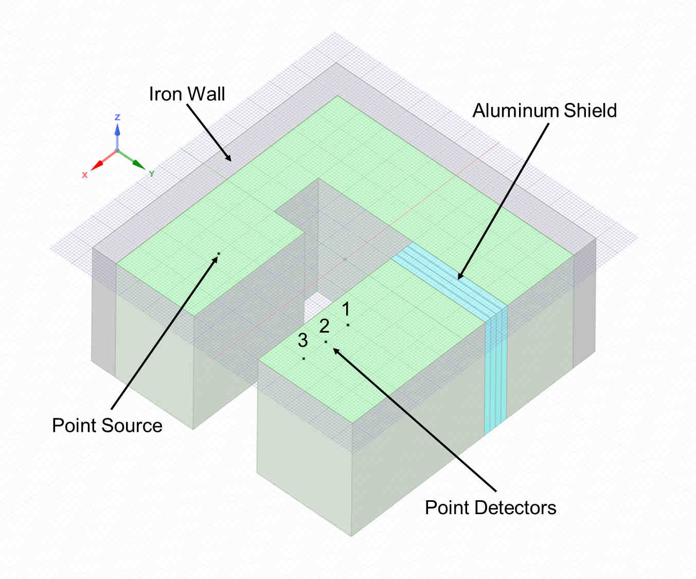
Figure 1. XY-cross section (z = -50 cm) of geometry showing the point source and point detector locations.
The problem is constructed such that particles can only reach the point detectors by first scattering off the iron shield on both the X and Y surfaces of the labyrinth, then passing through the aluminum shield. As a result, the contribution of the unscattered (primary) gammas to the detectors is 0. Coordinates of the source and detectors are provided in Table 1.

Table 1. Location Coordinates (cm) of Point Source and Detectors
The computational mesh contains 10419 elements. Attila deterministic solver calculations use the Transpire46g cross section set (46 gamma groups) in which all fine gamma groups above 1.35 MeV (the highest source energy group) are unassigned and groups below 1.15 MeV (the lowest source energy group) are collapsed by two. For the deterministic Attila solver calculations, an SN order of 20 and a Pn order of 3 are used.
A flux-to-dose conversion factor is used for Attila, Attila4MC, and MCNP-CSG to obtain comparable results and assume a normalized total source strength of 1 particle s-1. Importances were assigned in the Attila4MC calculation to match those from the legacy MCNP-CSG calculation. The deterministic Attila solver calculation is performed using the First Scattered Distributed Source (FSDS) capability with a quartic ray tracing style. Through the FSDS feature, the uncollided and collided (scattered) components of the solution are separately calculated, then merged to obtain the total flux solution. However, only the collided component is of interest in this calculation, so the merge step is deactivated. Collided flux is calculated at points with the use of the Mesh Based Last Collided method with a 56-point ray trace rule, which semi-analytically transports the last scattered flux to the associated edit points. Table 2 shows which calculations provide results for the various calculation methods. Attila-No LC are calculations in which the last collided method (LC) is not applied.

Table 2. Calculation File Index
Deterministic Attila solver calculations are run through the FSDS object in the GUI, labelled Run1-Attila-FSDS, which references the base Attila calculation, Run1-Attila. The Attila calculation results are located in the Run1-Attila-FSDS subdirectory, and separately include the uncollided (*uncol.) and collided (*coll.) components. The uncollided (unscattered) primary flux is expected to be equal to zero.
Contour plots of the primary (a) and scattered flux (b) from the deterministic Attila solver calculations are provided in Figure 2. A contour plot of the total flux from the Attila4MC calculation is shown in Figure 3.
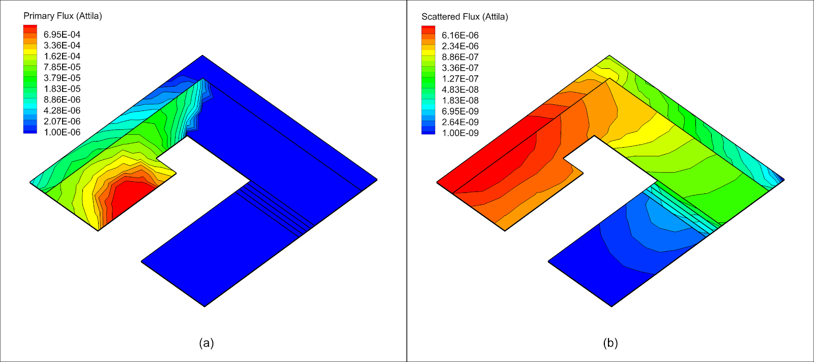
Figure 2. Contour plots of the primary (a) scattered (b) flux for the deterministic Attila solver calculations.
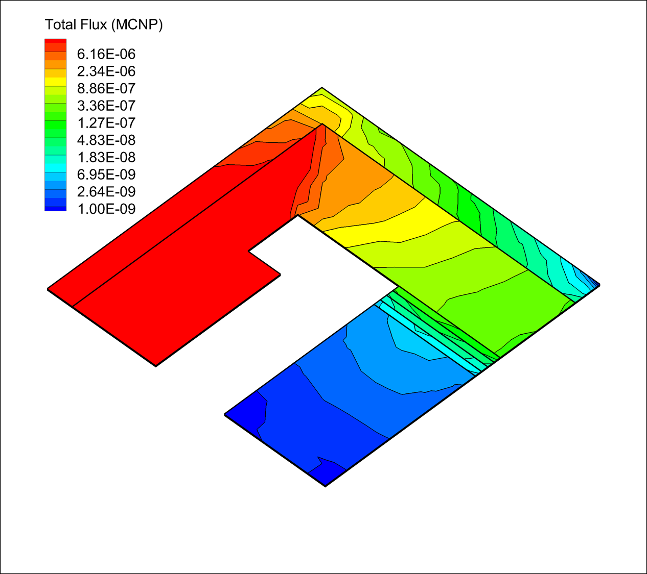
Figure 3. Contour plot of the total flux for the Attila4MC calculation.
Table 2 shows results using the four calculations methods (Attila-No LC, Attila-LC, Attila4MC, and MCNP-CSG). The Point (Edit) # is identical to the information listed in Table 1. Attila4MC calculations were run to convergence with a relative error of less than 5% (1.00E+07 histories for Attila4MC, 2.00E+07 histories for MCNP-CSG). Results can be obtained by running fewer histories. Ratios of Attila-No LC, Attila-LC, and MCNP-CSG to Attila4MC (Calculation Method/Attila4MC) results are included.

Table 2. Point Detector Results and Calculation Ratios (relative).